Definition of Price Elasticity of Demand(PED) from wikipedia

Price elasticity of demand (PED or Ed) is a measure used in economics to show the responsiveness, or elasticity, of the quantity demanded of a good or service to a change in its price, ceteris paribus. More precisely, it gives the percentage change in quantity demanded in response to a one percent change in price (ceteris paribus).

The R code below is a simple example of the Price elasticity analysis using a linear regression model.

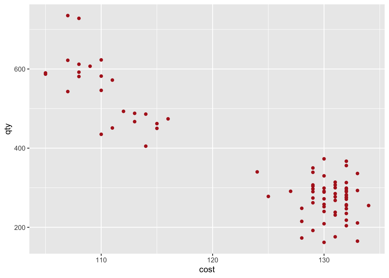
Here’s a visual of the example data.

To determine which variables are strongly correlated to qty sold, let’s use GGally’s ggpairs() function.

Final_Product_data %>% select(qty, cost, everything()) %>% ggpairs(lower = "blank")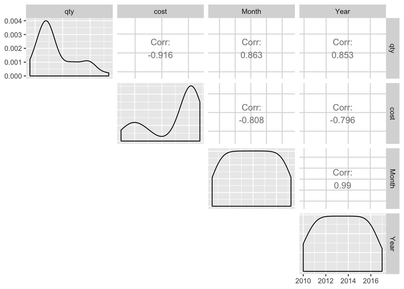

The magnitude of the correlation coeffs between qty and cost is the highest, followed by Month and Year, so a linear regression model can include all the variables.

Modeling

m.Final_product <- lm(qty ~ cost + Month, data = Final_Product_data)
sum_m.Final_product <- summary(m.Final_product)
sum_m.Final_product

## 
## Call:
## lm(formula = qty ~ cost + Month, data = Final_Product_data)
## 
## Residuals:
##      Min       1Q   Median       3Q      Max 
## -108.934  -29.140   -4.127   32.505  158.218 
## 
## Coefficients:
##              Estimate Std. Error t value Pr(>|t|)    
## (Intercept) 400.45221  306.89425   1.305    0.196    
## cost         -9.21379    0.95594  -9.638 5.54e-15 ***
## Month         0.06868    0.01264   5.436 5.90e-07 ***
## ---
## Signif. codes:  0 '***' 0.001 '**' 0.01 '*' 0.05 '.' 0.1 ' ' 1
## 
## Residual standard error: 48.59 on 79 degrees of freedom
## Multiple R-squared:  0.883,  Adjusted R-squared:   0.88 
## F-statistic: 298.1 on 2 and 79 DF,  p-value: < 2.2e-16

In this example, I have included only cost and Month variables with their P value at 5.543328910^{-15}, and 5.897822610^{-7} respectively, as they appear to be significant in affecting the volume of sale units.

We can try different model set-ups to find the best fit based on R2 and adjusted R2 values. Using functions in tidyverse/modelr/broom.

#Create List of models

formulas_for_lm <- list(
  prod_no_log <- qty ~cost + Month,
  prod_w_log <- log10(qty) ~ log10(cost) + Month
)

# Map the lm function to the list of formulas
Rsquared_fit_all <- formulas_for_lm %>% 
  map(lm, data = Final_Product_data) %>% 
  map_df(glance, .id = "model") %>% 
  select(model, r.squared, p.value)

#Display Rsquared 

Rsquared_fit_all

##   model r.squared      p.value
## 1     1 0.8829924 1.564806e-37
## 2     2 0.8656075 3.722364e-35

# 
slope_intercept_all <- formulas_for_lm %>% 
  map(lm, data = Final_Product_data) %>% 
  map_df(tidy, .id = "model") %>% 
  select(model, term, estimate, std.error)

slope_intercept_all

##   model        term      estimate    std.error
## 1     1 (Intercept)  4.004522e+02 3.068942e+02
## 2     1        cost -9.213787e+00 9.559375e-01
## 3     1       Month  6.868009e-02 1.263543e-02
## 4     2 (Intercept)  5.217442e+00 8.894790e-01
## 5     2 log10(cost) -2.157626e+00 3.232426e-01
## 6     2       Month  1.134625e-04 1.548824e-05

The best fit model appears to be model 1, so let us visualize the predicted values.

plot_model1 <- Final_Product_data %>% 
  add_predictions(m.Final_product) %>% 
  ggplot(aes(x = cost)) +
  geom_point(aes(y = qty), data = Final_Product_data, color = "firebrick") +
  geom_line(aes(y = pred))

plot_model1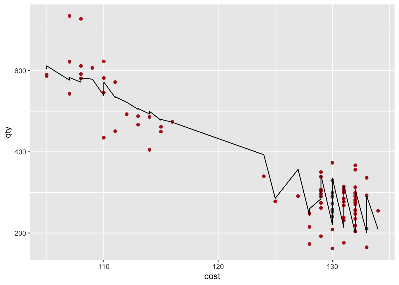

To estimate the PE, we will need the coefficient on cost \((\Delta Q/\Delta P)\) from the model, and the average cost & average quantity sold from the dataset:

• PED \(=(\Delta Q/\Delta P)*(\bar{P}/\bar{Q})\) where \(\Delta Q\) is change in quantity, \(\Delta P\) is change in price, \(\bar{P}\) is the avg price, and \(\bar{Q}\) is the avg quantity/sales Units.

PEcalc <- function(modelresult, df) {
  PE <- round(as.numeric(modelresult$coefficients[2] * (mean(df$cost)/mean(df$qty))),2)
  return(PE)
}

PEcalc(m.Final_product,Final_Product_data)

## [1] -3.25

The PE for the first model is -3.25, which shows that a 1% decrease in price will increase units sold by 3.25%. Or a 10% decrease in price will increase units sold by 32.5% and vice-versa.

Elasticity Interpretation:

• If PED < 1 (in absolute value), demand is inelastic (we will want to increase the price because changes in price have a relatively small effect on the quantity of good demanded)
• IF PED > 1 (in absolute value), demand is elastic (we will want to decrease the price because changes in price have a larger effect on the quantity or bigger percent change in demand)
• If PED == 1 (Rev is maximized )

The optimal price includes a “markup” proportional to the price elasticity of demand.

To find out the optimal price to maximize either revenue, or profit, we simplify the model output to:

options(scipen=999)

# x is the price

# Assume no marginal cost
equation_1_nocost = function(x) x*((m.Final_product$coefficients[[1]]) + PEcalc(m.Final_product,Final_Product_data)*x+ (m.Final_product$coefficients[[3]]))

opt_price_w_no_cost <- optimize(equation_1_nocost, c(50,140), maximum = TRUE)

# Assume $10 as marginal cost
equation_w_cost = function(x) (x-10)*((m.Final_product$coefficients[[1]]) + PEcalc(m.Final_product,Final_Product_data)*x+ (m.Final_product$coefficients[[3]]))

opt_price_w_cost <- optimize(equation_w_cost, c(50,100), maximum = TRUE)
The optimal price for maximizing profit is `r round(opt_price_w_cost[[1]],2)`; the maximum profit will be `$``r round(opt_price_w_cost[[2]],2)`

The optimal price for maximizing revenue is 61.62; the maximum revenue will be $12339.77.

Predict the sales for a particular month

data_w_new_price <- tibble(cost = opt_price_w_no_cost[[1]], Month = as.IDate("2017-07-01"))
predict(m.Final_product, data_w_new_price, interval = "p")

##        fit      lwr      upr
## 1 1024.174 888.1762 1160.171

Thanks to Allan Engelhardt for all his help on the analysis/thorough explanation of linear regression models, and the excellent and detailed Cross-Price_Elasticity article by Jack Han.