

This is Part 1 of a 3 Part series of predicting Customer Churn. Part 1 focuses on feature engineering, with the objective of deriving features that best represent drivers of churn.
Once the selected raw data is preprocessed, my first step towards the analysis starts with understanding how to frame data features with customers in mind; specifically, how can I transform data such that I am able to answer, say, what purchase/non-purchase customer behavior patterns tell their churn/no-churn story? Quantifying customer purchase behavior patterns, is one of the approaches that answers the question, and feature engineering produces the quantification parameters to output 2 useful products:
- Product 1: Quantitative Segmentation of our customers: Who are they?
- Product 2: Context-based Features to feed/help our predictive model: Which customers based on those features are likely to churn?
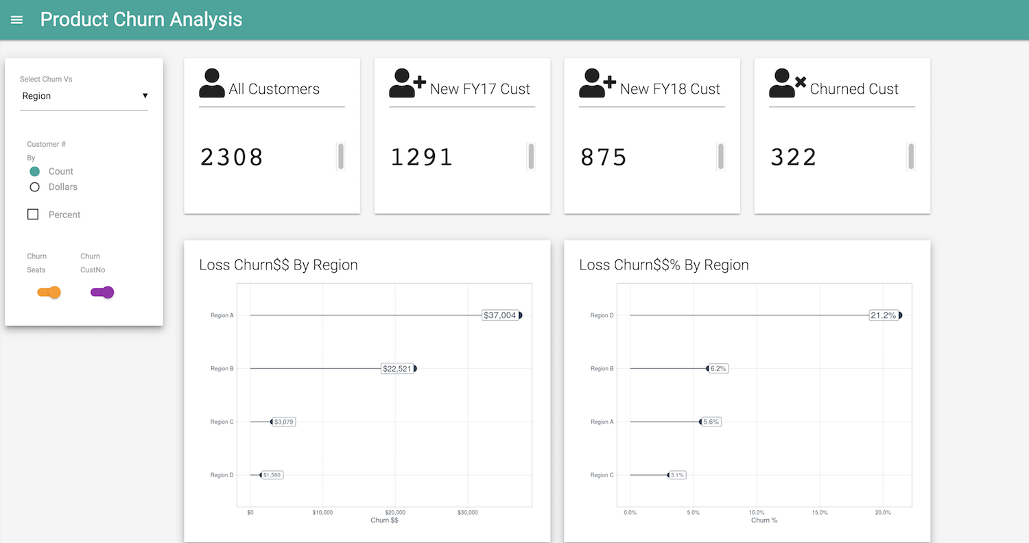
The output of the Analysis is available as an incremental shiny app here
2 notable feature engineering quotes.
Feature engineering is the process of transforming raw data into features that better represent the underlying problem to the predictive models, resulting in improved model accuracy on unseen data – Dr. Jason Brownlee
Coming up with features is difficult, time-consuming, and requires expert knowledge. ‘Applied machine learning’ is basically feature engineering — Andrew Ng
Part 1: Feature Engineering
Key Objective: Simplicity and Maintainability. Build Features that can be understood by the targeted human audience and best represents the problem to the predictive model.
- Start with feature selection to extract a relevant subset of the raw dataset. While correlation or other feature selection methods can be applied for feature selection, my first filter to selecting features are the Subject Matter Experts in the organisation(e.g. Product Owners/Sales) as the domain knowledge they contribute is one of the best filters for reducing noise in the data.
Let’s take a look at the example of a relevant subset of raw data using skimr.
skim(blog_raw_data)## Skim summary statistics
## n obs: 5195
## n variables: 12
##
## ── Variable type:character ──────────────────────────────────────────────────────────
## variable missing complete n min max empty n_unique
## Feature_Xtra 0 5195 5195 2 9 0 3
## Industry 0 5195 5195 10 10 0 12
## Payment Method 0 5195 5195 8 8 0 6
## Region 0 5195 5195 8 8 0 4
## Sales Person 0 5195 5195 6 8 0 7
## Ship Country 0 5195 5195 5 24 0 55
##
## ── Variable type:Date ───────────────────────────────────────────────────────────────
## variable missing complete n min max median n_unique
## Cal.Month 0 5195 5195 2016-07-01 2018-07-01 2017-09-01 25
##
## ── Variable type:numeric ────────────────────────────────────────────────────────────
## variable missing complete n mean sd p0 p25 p50 p75 p100
## ASP 0 5195 5195 10.17 3.07 -5 9 12 12 14
## Total_Amt 0 5195 5195 223.79 345.5 -172 96 144 240 9000
## Total_Qty 0 5195 5195 23.73 50.21 4 8 12 24 972
## hist
## ▁▁▁▁▂▁▁▇
## ▇▁▁▁▁▁▁▁
## ▇▁▁▁▁▁▁▁
##
## ── Variable type:POSIXct ────────────────────────────────────────────────────────────
## variable missing complete n min max median
## Maint End Date 0 5195 5195 2016-07-21 2019-09-13 2018-08-23
## Month 0 5195 5195 2016-07-01 2018-07-01 2017-09-01
## n_unique
## 764
## 25- Transform date-time variable to date-time with context features. For example, the date-time variable
Cal.Monthcan be used to engineer the month a customer purchased the product, the monthly cohort/s those particular customers belong to, and the tenure of the customers. Businesses usually look to gaining transaction/churn insights on a monthly, quarterly, yearly, andFiscal year(Fiscal Year in this example starts in July), so we can feature engineer those as well.
Feature_engineered_set1 <- blog_raw_data %>%
  mutate(quarter_year = as.yearqtr(Cal.Month),
         Year = year(Cal.Month),
         FY = (year(Cal.Month) + (month(Cal.Month) >=7)),
         Month_Purchased = month(Cal.Month),
         Monthly_cohort = month.abb[Month_Purchased],
         Month_Churn = month.abb[month(`Maint End Date`)]
        )

glimpse(Feature_engineered_set1)
## Observations: 5,195
## Variables: 18
## $ Month <dttm> 2017-01-01, 2017-01-01, 2017-01-01, 2017-01-01…
## $ Region <chr> "Region C", "Region C", "Region C", "Region C",…
## $ `Sales Person` <chr> "Online", "Online", "Online", "Online", "Online…
## $ Industry <chr> "Industry G", "Industry G", "Industry G", "Indu…
## $ `Ship Country` <chr> "Australia", "New Zealand", "Australia", "Austr…
## $ `Maint End Date` <dttm> 2017-06-11, 2017-11-20, 2018-01-10, 2017-10-12…
## $ `Payment Method` <chr> "Method_D", "Method_B", "Method_B", "Method_B",…
## $ Cal.Month <date> 2017-01-01, 2017-01-01, 2017-01-01, 2017-01-01…
## $ Total_Amt <dbl> 10, 40, 186, 36, 42, 96, 98, 96, 32, 34, 142, 3…
## $ Total_Qty <dbl> 4, 4, 16, 4, 4, 8, 12, 8, 4, 4, 16, 4, 20, 36, …
## $ ASP <dbl> 2, 10, 12, 9, 10, 12, 8, 12, 8, 8, 9, 10, 12, 1…
## $ Feature_Xtra <chr> "Feature_1", "Feature_1", "Feature_1", "Feature…
## $ quarter_year <yearqtr> 2017 Q1, 2017 Q1, 2017 Q1, 2017 Q1, 2017 Q1…
## $ Year <dbl> 2017, 2017, 2017, 2017, 2017, 2017, 2017, 2017,…
## $ FY <dbl> 2017, 2017, 2017, 2017, 2017, 2017, 2017, 2017,…
## $ Month_Purchased <dbl> 1, 1, 1, 1, 1, 1, 1, 1, 1, 1, 1, 1, 1, 1, 1, 1,…
## $ Monthly_cohort <chr> "Jan", "Jan", "Jan", "Jan", "Jan", "Jan", "Jan"…
## $ Month_Churn <chr> "Jun", "Nov", "Jan", "Oct", "Nov", "Jan", "Sep"…- Our target is to predict customers who will churn. The dataset does not come preloaded with churn information. So how do we determine if a customer has churned? In this particular example, a customer churns if they do not renew their service annually, or if they have passed the
Maint End Datevariable without renewing. So, we engineer the churn feature setting a churn_check_flag, and using the max function on the variableMaint End Date. If aMaint End Dateis not available, engineer feature/features that will help determine which customers have churned. For example, if the customer has not purchased more than once in 365 days, then the customer has churned.
#set churn_check_flag
churn_check_flag <- as.POSIXct("2018-09-30")
data_w_churn <- Feature_engineered_set1 %>%
  group_by(`Cust No`) %>%
  mutate(max = if_else(`Maint End Date` == max(`Maint End Date`), `Maint End Date`, as.Date.POSIXct(NA))) %>%
  drop_na() %>%
mutate(churn = if_else(max > churn_check_flag, "No", "Yes"))- Numeric: Engineer the frequency of purchase/s, the average amount spent per purchase, and when the customer first purchased calculated in days, or months, or year depending on what is required. These 3 features are also known as Recency, Frequency, and Monetary and used frequently in marketing to determine customer purchase behavior pattern. This requires date-time numeric calculation of
Cal.Monthandtime1provided. There’s the date-time feature that can be used to engineer to count the number of days the customer has been with us.
feature_engineered_data_set2 <- feature_engineered_data_set1 %>%
  group_by(`Cust No`) %>%
  mutate( tenure_days = round(as.numeric(difftime(time1 = time1,
                             time2 = Cal.Month,
                             units = "days"))),
         recency = min(tenure_days),
         first_purchase = max(tenure_days),
         frequency = n(),
         Monetary = round(mean(Total_Amt),0)
  )
Categorical with context: When a user selects an additional feature, the feature Xtra column gets a yes, if not a “no”. This is manual one-hot encoding.
Feature Crosses: Combining 2 or more categorical attributes into a single one, in this case between segments, churn, first purchase and monetary features; the interdependence of features allows us to build conjunctive features/products more useful to the predictive model than the features individually.
divider_segment <- median(feature_engineered_data_set2$monetary)

Churn_data_w_segments <- feature_engineered_data_set2%>%
  group_by(`Cust No`) %>%
  mutate( segment = case_when(
          churn == "No" & between(first_purchase, 730, max(first_purchase)) ~ "2+ Years Active",
          churn == "No" & between(first_purchase, 365, 729) ~ "1+ Years Active",
          churn == "No" & first_purchase < 365 ~ "New Active",
          churn == "Yes" ~ "Inactive"
         ),

         segment_monetary = case_when(
           segment == "2+ Years Active" & Monetary <= divider_segment ~ "2+ Years Active low Value",
           segment == "2+ Years Active" & Monetary > divider_segment ~ "2+ Years Active high Value",
           segment == "1+ Years Active" & Monetary <= divider_segment ~ "1+ Year Active low Value",
           segment == "1+ Years Active" & Monetary > divider_segment ~ "1+ Year Active high Value",
           segment == "New Active" & Monetary <= divider_segment ~ "New Active low Value",
           segment == "New Active" & Monetary > divider_segment ~ "New Active high Value",
           segment == "Inactive" & Monetary <= divider_segment ~ "Inactive low Value",
           segment == "Inactive" & Monetary > divider_segment ~ "Inactive high Value"
         )) %>%
select(`Cust No`, Month, CustNo,`Maint End Date`, max, churn, recency, first_purchase, Monetary, frequency, segment, segment_monetary, everything())- Binning/Bucketing: Bin the segments by recency and frequency to engineer segmented frequency and segmented recency as this assigns ranges for the numeric recency, frequency features into distinct buckets/bins.
# Bin the segmented by recency

seg.rec_class <- c("0-6 mos", "7-12 mos", "13-18 mos", "19-24 mos", "2+ Years")

#Need to remove customer ID as it will try to mutate per
RFM_Churn_data_w_segments <- Churn_data_w_segments[,-1] %>%
  mutate(seg.freq = ifelse(frequency == 1, "1",
                          ifelse(frequency == 2, "2",
                          ifelse(frequency == 3, "3",
                          ifelse(frequency == 4, "4",
                          ifelse(frequency == 5, "5", '5+'
                        )))))) %>%
   mutate(seg.rec = ifelse(between(recency, 0, 180), seg.rec_class[1],
                          ifelse(between(recency, 181, 365), seg.rec_class[2],
                          ifelse(between(recency, 366, 546), seg.rec_class[3],
                          ifelse(between(recency, 547, 730), seg.rec_class[4], seg.rec_class[5]
                          )))),
          seg.rec = fct_relevel(seg.rec, seg.rec_class))%>%
    mutate_if(is.character, as.factor)
For more on feature engineering and the iterative process of feature engineering, head to Dr.Jason Brownlee’s writeups.
Next (Part 2), we will address data imbalance as we move into the modeling phase of the churn.

Share this post
Twitter
Google+
Facebook
Reddit
LinkedIn
StumbleUpon
Pinterest
Email